The Three Wishes

Most people using Open GENIE will wish to do one of three things

Wish 1 - Access their data, either from a file or directly from the data acquisition electronics.

Wish 2 - Display their data on the screen and make a hardcopy on a printer.

Wish 3 - Manipulate their data, for example, to focus or normalise it.

These are described separately in the following sections, but first this….

A Simple Example

Below is a description of a simple Open GENIE session to access time of flight data taken on the High Resolution Powder Diffraction (HRPD) instrument which gives you some idea of the usage of Open GENIE commands.

Once Open GENIE is running, most people will wish to set up some defaults to allow easy access to files in the data area of the instrument they are using. If you always use one instrument, these defaults can be set up in a command file to be run automatically when Open GENIE starts. Normally Open GENIE looks for the file "genieinit.gcl" in your home directory, so the defaults can be placed in that file

>> set/disk "axplib$disk:"
Default disk: axplib$disk:
>> set/instrument "hrp"
Default instrument: hrp
>> set/directory "[OPENGENIE.GENIE.EXAMPLES.DATA]"
Default directory: [OPENGENIE.GENIE.EXAMPLES.DATA]
>> set/extension "raw"
Default filename extension: .raw

On UNIX, the commands for setting defaults are similar and use the appropriate syntax for UNIX file names, except no Set/Disk command is needed. However, on all operating systems it is essential to put string arguments in double quotes.

>> set/instrument "hrp"
Default instrument: hrp
>> set/directory "/usr/local/genie/examples/data/"
Default directory: /usr/local/genie/examples/data/
>> set/extension "raw"
Default filename extension: .raw

Any raw set of data can then be collected using the Assign command followed by the run number

>> assign 8639
Default input: /usr/local/genie/examples/data/hrp08639.raw

An alternative is to use the Set/File/Input command which explicitly sets the file to be used. For example,

>> Set/File/Input "/usr/local/genie/examples/data/hrp08639.raw"
Default input: /usr/local/genie/examples/data/hrp08639.raw

Now that the source for the data has been selected individual spectra can be extracted from the data set using the spectrum function, which can be normally abbreviated to "s".

>> w = s(7)
Reading spectrum 7 /usr/local/genie/examples/data/hrp08639.raw
>> noise = s(1)
Reading spectrum 1 /usr/local/genie/examples/data/hrp08639.raw
>> corrected = w - noise

Here the seventh spectrum is read into the workspace w. The first spectrum in the file is subtracted from the spectrum in w and the result is put into the workspace corrected. The corrected spectrum can now be displayed on a graph using the display command, and the binning number altered to 10

>> alter/binning 10
>> display corrected
Displayed using bin-grouping of 10

To plot the two original spectra on the same plot, but using different colours to show them clearly

>> alter/plotcolour $blue
>> plot noise
Plotted using bin-grouping of 10
>> alter/plotcolour $red
>> plot w
Plotted using bin-grouping of 10
>>

The plot produced is shown below.

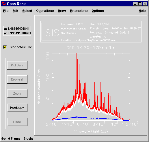
This brief example should have given you a good idea what an Open GENIE session looks like and a mental framework into which the more detailed information in the next three sections will fit. The data file plotted here is typically available in the "/usr/local/genie/examples/data" directory on UNIX or AXPLIB$DISK:[OPENGENIE.GENIE.EXAMPLES.DATA], and by changing the file locations in the example above, you can reproduce this plot. Note: when help is typed from within Open GENIE you will be told where Open GENIE is installed, and from that you can deduce the position of the examples directory.